Calibrate simulation parameters

library(RITHMS)

After loading your own dataset, we recommend performing a quick diagnosis to guide the choice of parameters in the holo_simu() simulation framework. This vignette aims to support users in calibrating simulations so that they better reflect the characteristics of their data.

We focus here on two parameters that influence the behavior of the simulation:

• The genetic effect size $\sigma_\beta$, which shapes the distribution of QTLs effects across microbiome. Note: The default value of this parameter is optimized to match the Deru dataset, wich sets it to 0.3.
• The multinomial sampling size parameter, used to perform the multinomial sampling step that converts abundances to counts data. Note: The default value of this parameter is optimized to match the Deru dataset, wich sets it to 10,000.

library(magrittr)
library(dplyr)
library(ggplot2)
library(ggrepel)
library(paletteer)
library(data.table)
library(glue)
library(plotly)
library(psych)

Calibrating the Genetic Effect Size

The genetic effect size parameter $\sigma_\beta$ directly impacts the distribution of taxa heritabilities (Further explanations are given in Pety et al. (2025) ). The gen_effect_calibration() function allows users to evaluate how different values of $\sigma_\beta$ influence this distribution.

In practice, heritabilities for most taxa are expected to lie around 0.1, rarely exceeding 0.5 as suggested in Zang et al. (2022) .

data(Deru)
ToyData <- Deru

taxa_assign_g <- assign_taxa(founder_object = ToyData)
effect_size_vector <- c(seq(0.1, 1, by = 0.1))
out_data <- gen_effect_calibration(founder_object = ToyData,
                                   taxa_assign_g = taxa_assign_g,
                                   correlation = 0.5,
                                   effect.size = effect_size_vector,
                                   plot = TRUE)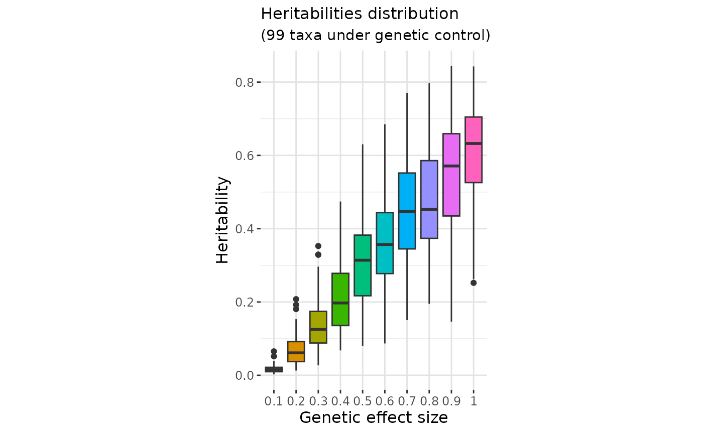

#> Picking joint bandwidth of 0.03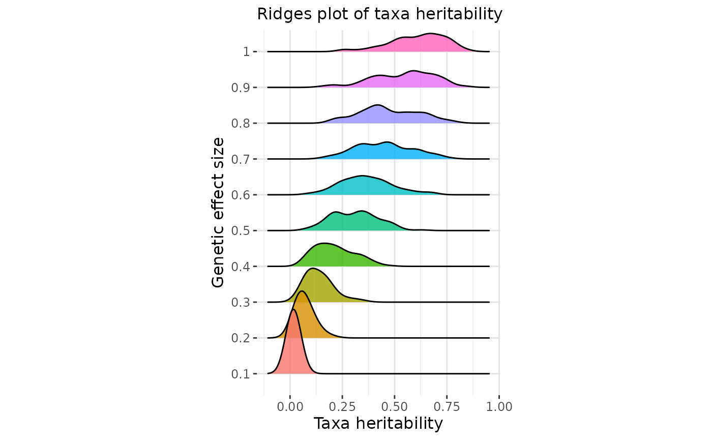6

Select effect sizes that lead to taxa heritability distributions consistent with the literature:

density_peaks <- out_data %>%
  group_by(effect.size) %>%
  summarise(
    peak = density(Heritability)$y[which.max(density(Heritability)$y)],
    peak_x = density(Heritability)$x[which.max(density(Heritability)$y)]
  )


out_data_filtered <- out_data %>% semi_join(density_peaks, by = "effect.size")

p2 <- ggplot(out_data_filtered, aes(x = Heritability, fill = as.factor(effect.size))) +
  geom_density(alpha = 0.5, color = NA) +
  geom_text(
    data = density_peaks,
    aes(x = peak_x, y = peak, label = as.factor(effect.size), color = as.factor(effect.size)),
    inherit.aes = FALSE,
    hjust = -0.1,
    size = 3,
    show.legend = FALSE
  ) +
  labs(
    x = "Taxa heritability",
    y = "Density",
    fill = "Genetic effect size",
    title = "Taxa heritability density, noise 0.5"
  ) +
  theme(
    panel.background = element_rect(fill = "white"),
    panel.grid.major = element_line(colour = "#e3e3e3"),
    panel.grid.minor = element_line(colour = "#e9e9e9"),
    axis.title = element_text(size = 8),
    axis.text = element_text(size = 7),
    plot.title = element_text(size = 7),
    legend.position = "right"
  ) +
  scale_fill_paletteer_d(paste0("werpals", "::", "uyuni")) +
  scale_color_paletteer_d(paste0("werpals", "::", "uyuni")) +
  guides(color = "none")

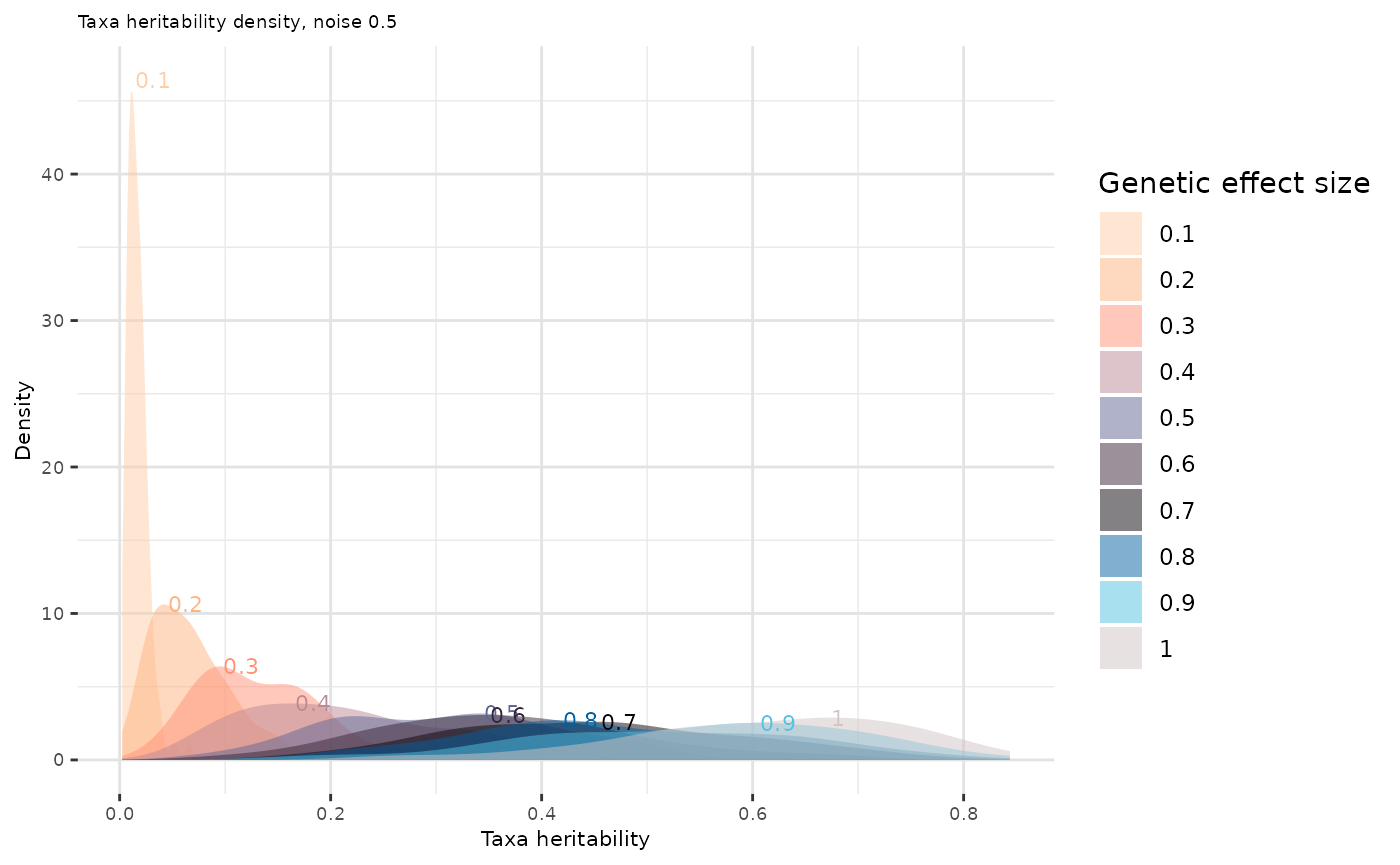
ggplotly(p2)

Based on the Zang et al. (2022) expectations, a reasonable distribution of taxa heritabilities appears to correspond to a value of $\sigma_\beta * \sqrt {QTL_o} = 0.3$ in the case of Déru et al. (2020) dataset.

Calibrating the Multinomial Sampling Size

The multinomial sampling size is used to simulate count data based on relative abundances, specially if the selection is based on diversity. The default value (10,000) in the richness_from_abundances_gen() function was calibrated using the Deru dataset and reflects its typical sequencing depths.

The counts are drawn according to a multinomial low such as $M(N,p)$ where $p$ is the relative abundances vector and $N$ the sampling size. Let the following formula $M(10000, (p_{i,1}, ..., p_{i,n_b}))$. This parameter should be adapted to your own dataset based on the observed sequencing depth distribution.

Sequencing depths distribution:

data(Deru)
ToyData <- Deru

sample_depth <- rowSums(ToyData$microbiome)

ggplot(data.frame(Depth = sample_depth), aes(x = Depth)) +
  geom_histogram(bins = 120, alpha = 0.3, fill = "#1f618d", color = "#1f618d") +
  labs(title = "Sequencing depths distribution of the microbiome",
       x = "Sequencing depth",
       y = "Number of samples") +
  
  theme_minimal() +
  theme(legend.title = element_blank())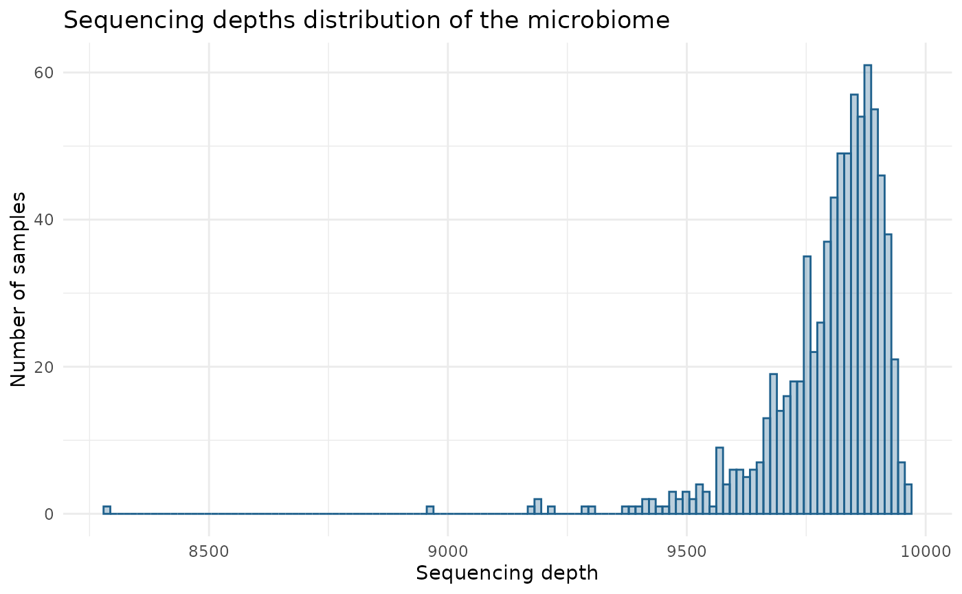

 
summary(sample_depth)
#>    Min. 1st Qu.  Median    Mean 3rd Qu.    Max. 
#>    8288    9753    9830    9798    9880    9965

We suggest using the median to promote robustness against potential outliers present in the dataset. In this example, the median is close to 10,000, supporting the default parameter value for this dataset.

Summary of parameter calibration

This vignette provides guidelines for calibrating these two parameters in the holo_simu() simulation framework based on a new dataset. These two parameters can be specified in the holo_simu() call, as well :

generations_simu <- holo_simu(founder_object = ToyData,
                              h2 = 0.25,
                              b2 = 0.25,
                              n_ind = 500,
                              n_clust = taxa_assign_g,
                              effect.size = 0.3,
                              size_rmultinom = 10000)

If you want to reproduce the figures in the article from your own dataset, remember to modify the size_rmultinom parameter of richness_from_abundances_gen() when computing diversity.

References

Déru, V., A. Bouquet, C. Hassenfratz, B. Blanchet, C. Carillier-Jacquin, and H. Gilbert. 2020. “Impact of a High-Fibre Diet on Genetic Parameters of Production Traits in Growing Pigs.” Animal 14 (11): 2236–45. https://doi.org/10.1017/s1751731120001275.

Pety, Solène, Mahendra Mariadassou, Ingrid David, and Andrea Rau. 2025. “RITHMS : An Advanced Stochastic Framework for the Simulation of Transgenerational Hologenomic Data.” https://doi.org/10.48550/ARXIV.2502.07366.

Zang, Xin-Wei, Hui-Zeng Sun, Ming-Yuan Xue, Zhe Zhang, Graham Plastow, Tianfu Yang, Le Luo Guan, and Jian-Xin Liu. 2022. “Heritable and Nonheritable Rumen Bacteria Are Associated with Different Characters of Lactation Performance of Dairy Cows.” Edited by Jessica L. Metcalf. mSystems 7 (5). https://doi.org/10.1128/msystems.00422-22.